ggposter: build an A1 conference poster from ggplot2

Toshikazu Matsumura

2026-07-08

Design

ggposter builds a poster declaratively: a theme controls colours, fonts and spacing; a title band spans the full width; and the rest of the poster is a set of columns, each a vertical stack of cards. A card is a rounded box with an accent-coloured header tab and one piece of content – text, a table, a ggplot figure, or a strip of photos. Every card is built as a plain [grid] grob, and the whole poster is assembled as one [gtable::gtable], so the same building blocks work whether the content is a bullet list or a ggplot.

Content and layout are described either as an R list, or as YAML read by [read_poster_yaml()]. Figures, tables, and photos referenced from the YAML are passed in separately as R objects (objects = list(...)), so the YAML stays purely declarative while data analysis stays in R.

library(ggposter)
library(ggplot2)

An example poster

The same mpg fuel-economy example used in the package README: a full-width title band and a two-column body of rounded, tab-headed cards for text, tables, figures, and a photo strip. It also shows height = "auto" (a card sized to fit its own content, instead of a fixed proportion of the column) and notes (a bullet-list description placed beside a table or figure):

tbl_class <- aggregate(cbind(hwy, cty) ~ class, data = mpg, FUN = function(x) round(mean(x), 1))
names(tbl_class) <- c("Class", "Mean hwy", "Mean cty")
class_best  <- tbl_class$Class[which.max(tbl_class$`Mean hwy`)]
class_worst <- tbl_class$Class[which.min(tbl_class$`Mean hwy`)]

tbl_drv <- aggregate(cbind(hwy, cty) ~ drv, data = mpg, FUN = function(x) round(mean(x), 1))
names(tbl_drv) <- c("Drivetrain", "Mean hwy", "Mean cty")
drv_best  <- tbl_drv$Drivetrain[which.max(tbl_drv$`Mean hwy`)]
drv_worst <- tbl_drv$Drivetrain[which.min(tbl_drv$`Mean hwy`)]

fig_facet <- ggplot(mpg, aes(displ, hwy, colour = class)) +
  geom_point() +
  labs(caption = paste(
    "• Highway mileage falls as engine displacement rises.",
    "• Compact and subcompact classes reach the highest mileage.",
    sep = "\n")) +
  theme_bw() +
  theme(legend.position = "inside", legend.position.inside = c(0.85, 0.72),
        legend.background = element_rect(fill = scales::alpha("white", 0.7), colour = NA),
        legend.key.size = unit(0.9, "lines"),
        plot.caption = element_text(hjust = 0, size = rel(1.3), colour = "black"))

fig_scatter <- ggplot(mpg, aes(cty, hwy, colour = drv)) +
  geom_point(alpha = 0.7) +
  theme_bw() +
  theme(legend.position = "inside", legend.position.inside = c(0.75, 0.32),
        legend.background = element_rect(fill = scales::alpha("white", 0.7), colour = NA))

fig_box <- ggplot(mpg, aes(drv, hwy, fill = drv)) +
  geom_boxplot(show.legend = FALSE) +
  labs(x = "Drivetrain", y = "Highway mpg") +
  theme_bw()
drv_med <- aggregate(hwy ~ drv, data = mpg, FUN = median)
drv_box_best <- as.character(drv_med$drv[which.max(drv_med$hwy)])

mpg_heat <- aggregate(hwy ~ class + drv, data = mpg, FUN = function(x) round(mean(x), 1))
fig_heat <- ggplot(mpg_heat, aes(drv, class, fill = hwy)) +
  geom_tile(colour = "white") +
  geom_text(aes(label = hwy), size = 2.6) +
  scale_fill_gradient(low = "#E8F5E9", high = "#2E7D32") +
  labs(x = "Drivetrain", y = "Class", fill = "Mean hwy") +
  theme_minimal() +
  theme(legend.position = "bottom")

img_dir <- system.file("extdata", package = "ggposter")
stock_photos <- c("small.JPG", "tall.jpg", "wide.jpg", "large.JPG")
stock_labels <- c("Photo A", "Photo B", "Photo C", "Photo D")

spec <- list(
  title = list(
    title = "Example Poster: Fuel Economy Patterns in the mpg Dataset",
    authors = "*Jane Doe (Example University), John Smith (Example Institute)",
    funding = "This is a demonstration poster for the ggposter package; it does not describe real research."
  ),
  layout = list(
    left  = c("objectives", "background", "methods", "summary_table", "fig_box", "fig_heat"),
    right = c("conclusions", "results_table", "fig_facet", "fig_scatter", "photos_2")
  ),
  sections = list(
    objectives = list(header = "OBJECTIVES", height = "auto", body = list(type = "text", md = c(
      "- Demonstrate the ggposter package.",
      "- Use the mpg fuel-economy dataset as example content.",
      "- Combine text, tables, figures, and photos in one poster."
    ))),
    background = list(header = "BACKGROUND", height = "auto", body = list(type = "text", md = c(
      "- Conference posters often mix text, tables, and figures.",
      "- ggposter arranges these as rounded, tab-headed cards.",
      "- Layout and content can be declared as an R list or a YAML file."
    ))),
    methods = list(header = "METHODS", height = "auto", body = list(type = "text", md = c(
      "- Data: the mpg dataset (234 vehicles, model years 1999-2008).",
      "- Figures: highway/city mileage by class and drivetrain.",
      "- Photos: generic stock images bundled with ggposter."
    ))),
    summary_table = list(header = "SUMMARY by class", height = "auto", body = list(
      type = "table", object = "tbl_class", title = "Mean mileage by vehicle class",
      notes = c(
        sprintf("- **%s** has the best highway mileage of all vehicle classes in this dataset.", class_best),
        sprintf("- **%s** has the worst, largely due to its greater size and weight.", class_worst),
        "- Compact and subcompact classes have nearly identical mean highway mileage.",
        "- Midsize vehicles average close to the compact/subcompact classes.",
        "- Pickup and SUV classes have the two lowest highway mileages, both under 19 mpg.",
        "- City mileage tracks highway mileage closely across all seven classes."
      )
    )),
    fig_box = list(header = "Mileage spread by drivetrain", height = "auto", body = list(
      type = "figure", object = "fig_box", notes_width = 0.4, height = 117,
      notes = c(
        "- Boxes show the full spread of highway mileage, not just the mean.",
        sprintf("- **%s**-wheel drive has the highest median highway mileage.", drv_box_best)
      )
    )),
    fig_heat = list(header = "Mean mileage: class x drivetrain", height = "auto", body = list(
      type = "figure", object = "fig_heat", notes_width = 0.4, height = 137,
      notes = c(
        "- Colour shows mean highway mpg for each class/drivetrain combination.",
        "- Blank cells are combinations that don't occur in the data."
      )
    )),
    conclusions = list(header = "CONCLUSIONS", height = "auto", body = list(type = "text", md = c(
      "- Compact and subcompact cars get the best highway mileage.",
      "- SUVs and pickups get the lowest.",
      "- ggposter can lay out this kind of summary automatically."
    ))),
    results_table = list(header = "SUMMARY by drivetrain", height = "auto", body = list(
      type = "table", object = "tbl_drv", title = "Mean mileage by drivetrain",
      notes = c(
        sprintf("- **%s**-wheel drive has the best highway mileage among the three drivetrain types.", drv_best),
        sprintf("- **%s**-wheel drive has the worst, mainly due to the added weight of the drivetrain.", drv_worst),
        "- The gap between front- and four-wheel drive is nearly 9 mpg highway."
      )
    )),
    fig_facet = list(header = "Mileage by class", height = "auto",
      body = list(type = "figure", object = "fig_facet", height = 280)),
    fig_scatter = list(header = "Highway vs. city mileage", height = "auto", body = list(
      type = "figure", object = "fig_scatter", notes_width = 0.45, height = 102,
      notes = c(
        "- Highway and city mileage are closely correlated.",
        "- 4-wheel drive vehicles cluster at the low-mileage end.",
        "- Front-wheel drive vehicles cluster at the high-mileage end."
      )
    )),
    photos_2 = list(header = "More sample photos", height = "auto", body = list(
      type = "image", files = stock_photos, labels = stock_labels,
      width = 230
    ))
  )
)

p <- poster(
  spec,
  objects = list(tbl_class = tbl_class, tbl_drv = tbl_drv,
                 fig_facet = fig_facet, fig_scatter = fig_scatter,
                 fig_box = fig_box, fig_heat = fig_heat),
  theme = theme_green(base_size = 24),
  base_dir = img_dir
)

p is a ggposter object – a thin wrapper around the assembled gtable. Font sizes and spacing are absolute physical measurements sized for the poster’s true paper size, so previewing at an arbitrary plot size (as this vignette must) needs a scaled-down render rather than printing p directly:

render_poster(p, "ggposter-minimal-preview.png", scale = 0.3, dpi = 150)
knitr::include_graphics("ggposter-minimal-preview.png")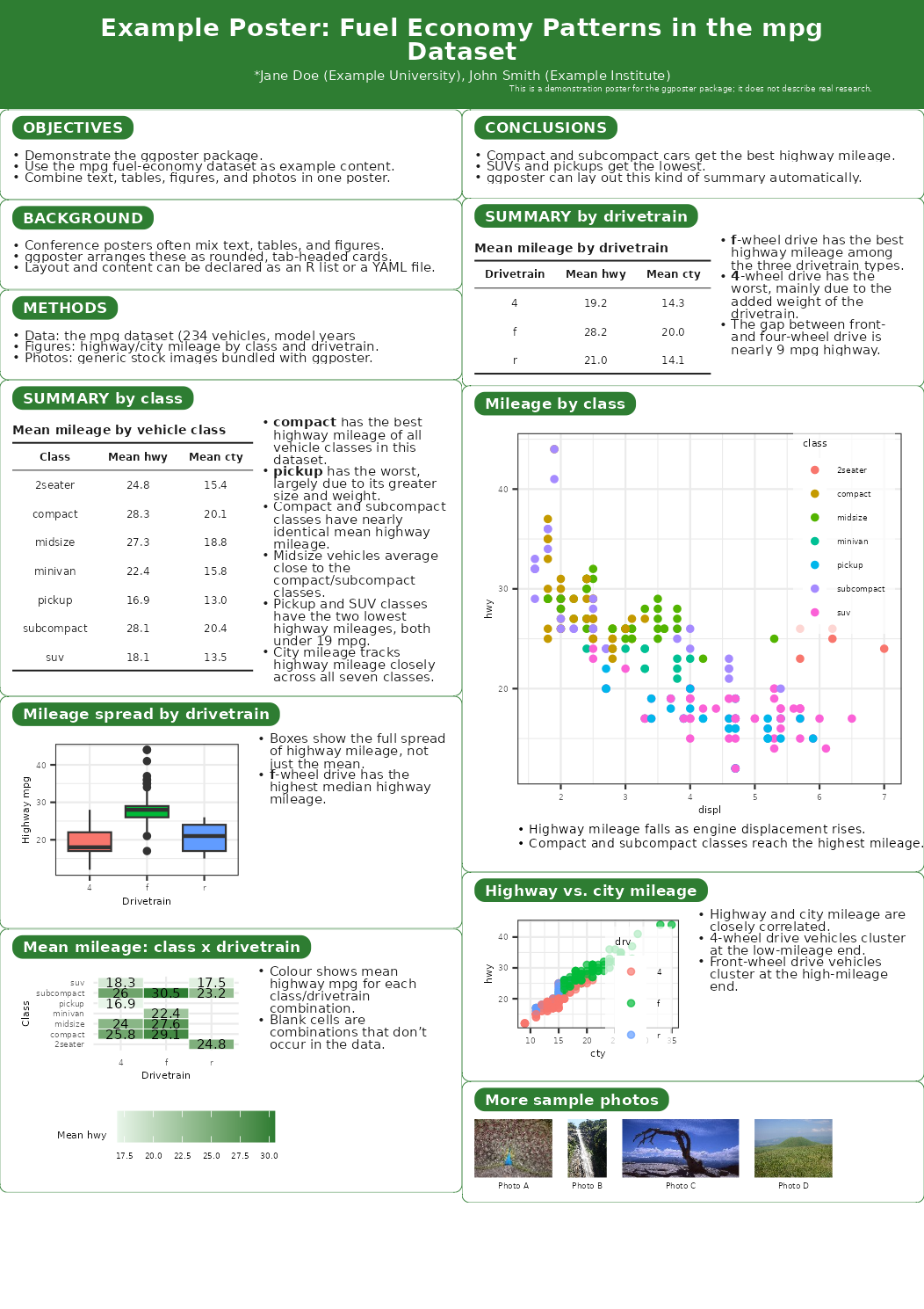

Save it at true size with [render_poster()]:

render_poster(p, "poster.pdf")          # true A1 size, fonts embedded
render_poster(p, "preview.png", scale = 0.25, dpi = 150)  # A4-ish preview

Content types

Every section has a header (or NULL for no header) and a body with a type:

• "text" – a character vector of markdown-ish lines, rendered via [card_text()]. Lines starting with "- " become bulleted.
• "table" – a data.frame/tibble named in objects, rendered via [card_table()] as a booktab-style table with an optional title/caption. The table’s font size is shrunk automatically to fit the column.
• "figure" – a ggplot object named in objects, rendered via [card_figure()], re-themed to the poster’s base font size/family.
• "image" – one or more photo files, rendered via [card_image()] as a labelled row (e.g. a “dominant species” photo band).

Theming

[poster_theme()] controls the accent colour, fonts, corner radius, and spacing; [theme_green()] is a ready-made preset. Latin and CJK (Japanese) fonts are set independently, and [poster_font()] picks an installed family automatically so PDF export embeds real glyphs rather than falling back to a substitute:

th <- theme_green(base_size = 24, base_family = poster_font())
th
#> 
#> ── poster_theme ────────────────────────────────────────────────────────────────
#> accent: #2E7D32
#> box_fill: #FFFFFF
#> box_border: #2E7D32
#> base_family: DejaVu Sans
#> cjk_family: DejaVu Sans
#> base_size: 24 pt

# For a Japanese poster, pick an installed CJK-capable family:
th_jp <- poster_theme(base_family = poster_font(cjk = TRUE))

Reproducing a real poster

The following reproduces the layout and text of a real conference poster (poster.pdf in this package’s development repository): a full-width title band and a two-column body of rounded, tab-headed cards for the introduction/background/methods on the left and conclusions/results on the right.

The title, author list, funding note, and all body text and tables are transcribed verbatim from the original poster. The cutting-regime scatterplot and the community ordination plot are illustrative, generated from the reported per-community means and standard deviations (not the original point-level field data, which is not published in the poster). The photos are generic stock images bundled with the package, standing in for the original species photographs.

tbl_courses <- tibble::tribble(
  ~`Golf course`, ~`Established year`, ~`Area (ha)`, ~`Total grassland spp.`,
  ~`Grassland spp. (mean +/- SD /m2)`, ~`All spp. (mean +/- SD /m2)`,
  "A", 1903, 20, 79, "6.5 +/- 2.8", "11.2 +/- 4.6",
  "B", 1926, 70, 55, "2.9 +/- 2.0", "5.2 +/- 4.6",
  "C", 1930, 55, 78, "4.4 +/- 2.8", "8.1 +/- 5.1",
  "D", 1956, 60, 55, "2.1 +/- 1.5", "4.0 +/- 3.3"
)

tbl_community <- tibble::tribble(
  ~Community, ~`No. of plots`, ~`Grassland spp. (/m2)`, ~`All spp. (/m2)`,
  ~`Cutting height (cm)`, ~`Cutting freq. (/yr)`, ~`Main dominant species`,
  "com1", 57, "6.1 +/- 2.9", "10.7 +/- 4.7", "12.9 +/- 15.3", "4.2 +/- 6.1",
    "P. chino var. viridis, A. hirta, M. sinensis",
  "com2", 38, "5.3 +/- 2.7", "10.6 +/- 5.2", "22.7 +/- 19.2", "4.4 +/- 4.4",
    "P. chino var. viridis, I. cylindrica var. koenigii",
  "com3", 37, "3.9 +/- 1.3", "6.9 +/- 3.1",  "5.1 +/- 4.8",   "10.1 +/- 5.3",
    "Z. aponica, I. cylindrica var. koenigii",
  "com4", 68, "1.4 +/- 0.7", "2.4 +/- 1.6",  "5.2 +/- 5.0",   "14.6 +/- 5.5",
    "Z. aponica"
)

set.seed(42)
community_params <- tibble::tribble(
  ~Community, ~n, ~height_mean, ~height_sd, ~freq_mean, ~freq_sd,
  "com1", 57, 12.9, 15.3, 4.2, 6.1,
  "com2", 38, 22.7, 19.2, 4.4, 4.4,
  "com3", 37, 5.1,  4.8,  10.1, 5.3,
  "com4", 68, 5.2,  5.0,  14.6, 5.5
)

# illustrative points matching the reported mean +/- SD, not raw field data
df_cutting <- purrr::list_rbind(purrr::pmap(community_params, function(Community, n,
                                                          height_mean, height_sd,
                                                          freq_mean, freq_sd) {
  tibble::tibble(
    Community = Community,
    cutting_height = pmax(0, rnorm(n, height_mean, height_sd)),
    cutting_freq   = pmax(1, rnorm(n, freq_mean, freq_sd))
  )
}))
fig_cutting <- ggplot(df_cutting, aes(cutting_freq, cutting_height)) +
  geom_point(alpha = 0.6, colour = "#2E7D32") +
  facet_wrap(~Community, nrow = 1) +
  labs(x = "Cutting frequency (/yr)", y = "Cutting height (cm)") +
  theme_bw()

df_ord <- purrr::list_rbind(purrr::pmap(community_params, function(Community, n, ...) {
  centre <- switch(Community,
    com1 = c(1, 1), com2 = c(1, -1), com3 = c(-1, 0.5), com4 = c(-1.2, -1))
  tibble::tibble(Community = Community,
                 NMDS1 = rnorm(n, centre[1], 0.4),
                 NMDS2 = rnorm(n, centre[2], 0.4))
}))
fig_ordination <- ggplot(df_ord, aes(NMDS1, NMDS2, colour = Community)) +
  geom_point(alpha = 0.7) +
  stat_ellipse() +
  theme_bw() +
  theme(legend.position = "bottom")

The layout, theme, and section text live in a YAML file bundled with the package:

yml_path <- system.file("extdata", "poster_sample.yml", package = "ggposter")
cat(readLines(yml_path)[1:20], sep = "\n")
poster:
  size: A1
  orientation: portrait

theme:
  accent: "#2E7D32"
  base_size: 24

title:
  title: "The relationship between grassland species richness and the management in long-established golf courses in Japan"
  authors: "*Toshikazu Matsumura (Konan Women's Univ.), Yoshinobu Hashimoto (Museum of Nature and Human activities, Hyogo), Yoshihiro Sawada (Awaji Landscape Planning & Horticulture Academy / Univ. of Hyogo)"
  funding: "This study was supported by JSPS KAKENHI Grant Number 15K07833. We wish to thank the golf courses for field investigations."

layout:
  left:  [objectives, backgrounds, methods, course_summary, dominant_species]
  right: [conclusions, community_table, community_figure, ordination, other_species]

sections:
  objectives:
    header: "OBJECTIVES"

Assembling and rendering:

sample_poster <- poster(
  yml_path,
  objects = list(
    tbl_courses = tbl_courses, tbl_community = tbl_community,
    fig_cutting = fig_cutting, fig_ordination = fig_ordination
  ),
  theme = theme_green(base_size = 24),
  base_dir = dirname(yml_path)
)

render_poster(sample_poster, "ggposter-sample-preview.png", scale = 0.3, dpi = 150)
knitr::include_graphics("ggposter-sample-preview.png")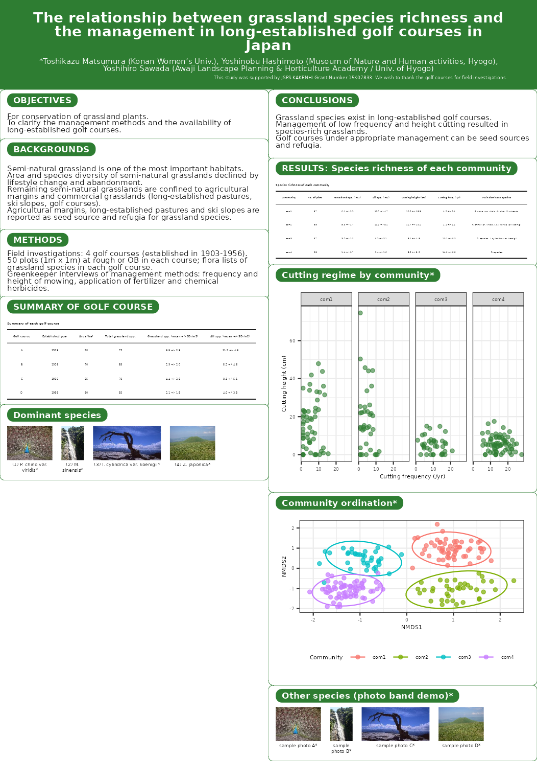

render_poster(sample_poster, "sample_poster.pdf")