The goal of ecan is to support ecological analysis.
Installation
The released version is available on CRAN.
install.packages("ecan")The development version on GitHub (branch main) is ahead of the version on CRAN, so the two do not match. It already includes features that are not released yet, such as twinspan() and its helpers. Install it if you need them.
  # install.packages("remotes")
remotes::install_github("matutosi/ecan")
You can use almost the same functionality in shiny.
Example
You can read docs in https://matutosi.github.io/ecan/
Prepare and convert data
library(ecan)
library(vegan)
#> Loading required package: permute
library(dplyr)
#>
#> Attaching package: 'dplyr'
#> The following objects are masked from 'package:stats':
#>
#>     filter, lag
#> The following objects are masked from 'package:base':
#>
#>     intersect, setdiff, setequal, union
library(stringr)
library(tibble)
library(ggplot2)
data(dune)
data(dune.env)

df <-
  table2df(dune) %>%
  dplyr::left_join(tibble::rownames_to_column(dune.env, "stand"))
#> Joining with `by = join_by(stand)`

sp_dammy <-
 tibble::tibble("species" = colnames(dune),
                "dammy_1" = stringr::str_sub(colnames(dune), 1, 1),
                "dammy_6" = stringr::str_sub(colnames(dune), 6, 6))

df <-
  df %>%
  dplyr::left_join(sp_dammy)
#> Joining with `by = join_by(species)`

df
#> # A tibble: 197 × 10
#>    stand species  abundance    A1 Moisture Management Use      Manure dammy_1
#>    <chr> <chr>        <dbl> <dbl> <ord>    <fct>      <ord>    <ord>  <chr>
#>  1 1     Achimill         1   2.8 1        SF         Haypastu 4      A
#>  2 1     Elymrepe         4   2.8 1        SF         Haypastu 4      E
#>  3 1     Lolipere         7   2.8 1        SF         Haypastu 4      L
#>  4 1     Poaprat          4   2.8 1        SF         Haypastu 4      P
#>  5 1     Poatriv          2   2.8 1        SF         Haypastu 4      P
#>  6 2     Achimill         3   3.5 1        BF         Haypastu 2      A
#>  7 2     Alopgeni         2   3.5 1        BF         Haypastu 2      A
#>  8 2     Bellpere         3   3.5 1        BF         Haypastu 2      B
#>  9 2     Bromhord         4   3.5 1        BF         Haypastu 2      B
#> 10 2     Elymrepe         4   3.5 1        BF         Haypastu 2      E
#> # ℹ 187 more rows
#> # ℹ 1 more variable: dammy_6 <chr>
Diversity index
div <-
  shdi(df) %>%
  dplyr::left_join(select_one2multi(df, "stand"))
#> Joining with `by = join_by(stand)`

group <- "Management"
div_index <- "s"
div %>%
  ggplot(aes(x = .data[[group]], y = .data[[div_index]])) +
    geom_boxplot(outlier.shape = NA) +  # do not show outer point
    geom_jitter(height = 0, width = 0.1)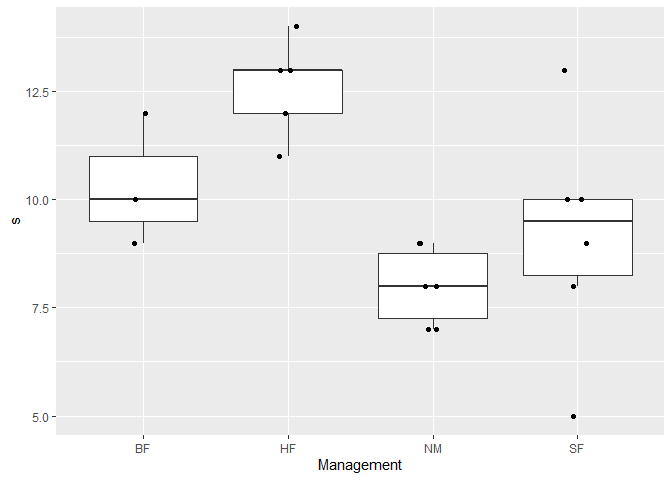
Indicator Species Analysis (ISA, ind val)
ind_val(df, group = "Moisture", row_data = TRUE)
#> $relfrq
#>                  1    2         3   4
#> Achimill 0.7142857 0.50 0.0000000 0.0
#> Elymrepe 0.4285714 0.50 0.0000000 0.5
#> Lolipere 1.0000000 0.75 0.1428571 0.5
#> Poaprat  1.0000000 1.00 0.2857143 0.5
#> Poatriv  0.7142857 0.75 0.4285714 1.0
#> Alopgeni 0.1428571 0.50 0.4285714 1.0
#> Bellpere 0.4285714 0.75 0.0000000 0.0
#> Bromhord 0.4285714 0.50 0.0000000 0.0
#> Scorautu 0.8571429 1.00 0.8571429 1.0
#> Trifrepe 0.8571429 0.75 0.7142857 1.0
#> Agrostol 0.0000000 0.50 0.8571429 1.0
#> Bracruta 0.7142857 0.75 0.7142857 1.0
#> Cirsarve 0.0000000 0.25 0.0000000 0.0
#> Sagiproc 0.1428571 0.25 0.4285714 1.0
#> Anthodor 0.4285714 0.50 0.1428571 0.0
#> Planlanc 0.7142857 0.50 0.0000000 0.0
#> Rumeacet 0.4285714 0.00 0.0000000 1.0
#> Trifprat 0.4285714 0.00 0.0000000 0.0
#> Juncbufo 0.1428571 0.00 0.1428571 1.0
#> Eleopalu 0.0000000 0.00 0.7142857 0.0
#> Juncarti 0.0000000 0.00 0.5714286 0.5
#> Ranuflam 0.0000000 0.00 0.8571429 0.0
#> Vicilath 0.2857143 0.25 0.0000000 0.0
#> Hyporadi 0.1428571 0.25 0.1428571 0.0
#> Chenalbu 0.0000000 0.00 0.1428571 0.0
#> Comapalu 0.0000000 0.00 0.2857143 0.0
#> Callcusp 0.0000000 0.00 0.4285714 0.0
#> Airaprae 0.0000000 0.25 0.1428571 0.0
#> Salirepe 0.1428571 0.00 0.2857143 0.0
#> Empenigr 0.0000000 0.00 0.1428571 0.0
#>
#> $relabu
#>                   1         2          3          4
#> Achimill 0.48780488 0.5121951 0.00000000 0.00000000
#> Elymrepe 0.25531915 0.2978723 0.00000000 0.44680851
#> Lolipere 0.46204620 0.3927393 0.05280528 0.09240924
#> Poaprat  0.35036496 0.3576642 0.08759124 0.20437956
#> Poatriv  0.24806202 0.2713178 0.15503876 0.32558140
#> Alopgeni 0.02846975 0.2241993 0.19928826 0.54804270
#> Bellpere 0.40000000 0.6000000 0.00000000 0.00000000
#> Bromhord 0.39506173 0.6049383 0.00000000 0.00000000
#> Scorautu 0.33922261 0.2226148 0.24028269 0.19787986
#> Trifrepe 0.27636364 0.2290909 0.18909091 0.30545455
#> Agrostol 0.00000000 0.2818792 0.38926174 0.32885906
#> Bracruta 0.29197080 0.1532847 0.24817518 0.30656934
#> Cirsarve 0.00000000 1.0000000 0.00000000 0.00000000
#> Sagiproc 0.05161290 0.2258065 0.18064516 0.54193548
#> Anthodor 0.33333333 0.5185185 0.14814815 0.00000000
#> Planlanc 0.70588235 0.2941176 0.00000000 0.00000000
#> Rumeacet 0.50000000 0.0000000 0.00000000 0.50000000
#> Trifprat 1.00000000 0.0000000 0.00000000 0.00000000
#> Juncbufo 0.06060606 0.0000000 0.09090909 0.84848485
#> Eleopalu 0.00000000 0.0000000 1.00000000 0.00000000
#> Juncarti 0.00000000 0.0000000 0.50000000 0.50000000
#> Ranuflam 0.00000000 0.0000000 1.00000000 0.00000000
#> Vicilath 0.63157895 0.3684211 0.00000000 0.00000000
#> Hyporadi 0.19047619 0.3333333 0.47619048 0.00000000
#> Chenalbu 0.00000000 0.0000000 1.00000000 0.00000000
#> Comapalu 0.00000000 0.0000000 1.00000000 0.00000000
#> Callcusp 0.00000000 0.0000000 1.00000000 0.00000000
#> Airaprae 0.00000000 0.5384615 0.46153846 0.00000000
#> Salirepe 0.27272727 0.0000000 0.72727273 0.00000000
#> Empenigr 0.00000000 0.0000000 1.00000000 0.00000000
#>
#> $indval
#>                    1          2           3          4
#> Achimill 0.348432056 0.25609756 0.000000000 0.00000000
#> Elymrepe 0.109422492 0.14893617 0.000000000 0.22340426
#> Lolipere 0.462046205 0.29455446 0.007543612 0.04620462
#> Poaprat  0.350364964 0.35766423 0.025026069 0.10218978
#> Poatriv  0.177187154 0.20348837 0.066445183 0.32558140
#> Alopgeni 0.004067107 0.11209964 0.085409253 0.54804270
#> Bellpere 0.171428571 0.45000000 0.000000000 0.00000000
#> Bromhord 0.169312169 0.30246914 0.000000000 0.00000000
#> Scorautu 0.290762241 0.22261484 0.205956588 0.19787986
#> Trifrepe 0.236883117 0.17181818 0.135064935 0.30545455
#> Agrostol 0.000000000 0.14093960 0.333652924 0.32885906
#> Bracruta 0.208550574 0.11496350 0.177267987 0.30656934
#> Cirsarve 0.000000000 0.25000000 0.000000000 0.00000000
#> Sagiproc 0.007373272 0.05645161 0.077419355 0.54193548
#> Anthodor 0.142857143 0.25925926 0.021164021 0.00000000
#> Planlanc 0.504201681 0.14705882 0.000000000 0.00000000
#> Rumeacet 0.214285714 0.00000000 0.000000000 0.50000000
#> Trifprat 0.428571429 0.00000000 0.000000000 0.00000000
#> Juncbufo 0.008658009 0.00000000 0.012987013 0.84848485
#> Eleopalu 0.000000000 0.00000000 0.714285714 0.00000000
#> Juncarti 0.000000000 0.00000000 0.285714286 0.25000000
#> Ranuflam 0.000000000 0.00000000 0.857142857 0.00000000
#> Vicilath 0.180451128 0.09210526 0.000000000 0.00000000
#> Hyporadi 0.027210884 0.08333333 0.068027211 0.00000000
#> Chenalbu 0.000000000 0.00000000 0.142857143 0.00000000
#> Comapalu 0.000000000 0.00000000 0.285714286 0.00000000
#> Callcusp 0.000000000 0.00000000 0.428571429 0.00000000
#> Airaprae 0.000000000 0.13461538 0.065934066 0.00000000
#> Salirepe 0.038961039 0.00000000 0.207792208 0.00000000
#> Empenigr 0.000000000 0.00000000 0.142857143 0.00000000
#>
#> $maxcls
#> Achimill Elymrepe Lolipere  Poaprat  Poatriv Alopgeni Bellpere Bromhord
#>        1        4        1        2        4        4        2        2
#> Scorautu Trifrepe Agrostol Bracruta Cirsarve Sagiproc Anthodor Planlanc
#>        1        4        3        4        2        4        2        1
#> Rumeacet Trifprat Juncbufo Eleopalu Juncarti Ranuflam Vicilath Hyporadi
#>        4        1        4        3        3        3        1        2
#> Chenalbu Comapalu Callcusp Airaprae Salirepe Empenigr
#>        3        3        3        2        3        3
#>
#> $indcls
#>   Achimill   Elymrepe   Lolipere    Poaprat    Poatriv   Alopgeni   Bellpere
#> 0.34843206 0.22340426 0.46204620 0.35766423 0.32558140 0.54804270 0.45000000
#>   Bromhord   Scorautu   Trifrepe   Agrostol   Bracruta   Cirsarve   Sagiproc
#> 0.30246914 0.29076224 0.30545455 0.33365292 0.30656934 0.25000000 0.54193548
#>   Anthodor   Planlanc   Rumeacet   Trifprat   Juncbufo   Eleopalu   Juncarti
#> 0.25925926 0.50420168 0.50000000 0.42857143 0.84848485 0.71428571 0.28571429
#>   Ranuflam   Vicilath   Hyporadi   Chenalbu   Comapalu   Callcusp   Airaprae
#> 0.85714286 0.18045113 0.08333333 0.14285714 0.28571429 0.42857143 0.13461538
#>   Salirepe   Empenigr
#> 0.20779221 0.14285714
#>
#> $pval
#> Achimill Elymrepe Lolipere  Poaprat  Poatriv Alopgeni Bellpere Bromhord
#>    0.264    0.441    0.076    0.344    0.512    0.059    0.110    0.198
#> Scorautu Trifrepe Agrostol Bracruta Cirsarve Sagiproc Anthodor Planlanc
#>    0.823    0.676    0.366    0.613    0.300    0.073    0.326    0.096
#> Rumeacet Trifprat Juncbufo Eleopalu Juncarti Ranuflam Vicilath Hyporadi
#>    0.093    0.136    0.002    0.023    0.206    0.002    0.703    1.000
#> Chenalbu Comapalu Callcusp Airaprae Salirepe Empenigr
#>    1.000    0.437    0.078    0.752    0.600    1.000
#>
#> $error
#> [1] 0
#>
#> attr(,"class")
#> [1] "indval"
ind_val(df, group = "Management")
#> Joining with `by = join_by(numeric_Management)`
#> # A tibble: 30 × 4
#>    Management species  ind.val p.value
#>    <fct>      <chr>      <dbl>   <dbl>
#>  1 SF         Alopgeni   0.547   0.036
#>  2 SF         Agrostol   0.472   0.063
#>  3 SF         Sagiproc   0.241   0.525
#>  4 SF         Elymrepe   0.188   0.703
#>  5 SF         Cirsarve   0.167   1
#>  6 SF         Chenalbu   0.167   1
#>  7 BF         Vicilath   0.571   0.034
#>  8 BF         Lolipere   0.45    0.071
#>  9 BF         Bromhord   0.448   0.046
#> 10 BF         Trifrepe   0.439   0.065
#> # ℹ 20 more rows
ind_val(df, group = "Use")
#> Joining with `by = join_by(numeric_Use)`
#> # A tibble: 30 × 4
#>    Use      species  ind.val p.value
#>    <ord>    <chr>      <dbl>   <dbl>
#>  1 Haypastu Poatriv    0.451   0.116
#>  2 Haypastu Alopgeni   0.359   0.201
#>  3 Haypastu Elymrepe   0.292   0.314
#>  4 Haypastu Poaprat    0.288   0.819
#>  5 Haypastu Agrostol   0.269   0.587
#>  6 Haypastu Lolipere   0.259   0.801
#>  7 Haypastu Sagiproc   0.178   0.799
#>  8 Haypastu Cirsarve   0.125   1
#>  9 Haypastu Chenalbu   0.125   1
#> 10 Haypastu Juncbufo   0.118   0.834
#> # ℹ 20 more rows
ind_val(df, group = "Manure")
#> Joining with `by = join_by(numeric_Manure)`
#> # A tibble: 30 × 4
#>    Manure species  ind.val p.value
#>    <ord>  <chr>      <dbl>   <dbl>
#>  1 4      Elymrepe   0.5     0.039
#>  2 4      Lolipere   0.351   0.194
#>  3 4      Cirsarve   0.333   0.294
#>  4 4      Poaprat    0.315   0.279
#>  5 4      Bellpere   0.248   0.474
#>  6 2      Rumeacet   0.522   0.038
#>  7 2      Trifprat   0.389   0.165
#>  8 2      Achimill   0.309   0.278
#>  9 2      Poatriv    0.299   0.432
#> 10 2      Anthodor   0.178   0.761
#> # ℹ 20 more rows
Cluster analysis
library(ggdendro)
library(dendextend)
#> Registered S3 method overwritten by 'dendextend':
#>   method     from
#>   rev.hclust vegan
#>
#> ---------------------
#> Welcome to dendextend version 1.19.1
#> Type citation('dendextend') for how to cite the package.
#>
#> Type browseVignettes(package = 'dendextend') for the package vignette.
#> The github page is: https://github.com/talgalili/dendextend/
#>
#> Suggestions and bug-reports can be submitted at: https://github.com/talgalili/dendextend/issues
#> You may ask questions at stackoverflow, use the r and dendextend tags:
#>   https://stackoverflow.com/questions/tagged/dendextend
#>
#>  To suppress this message use:  suppressPackageStartupMessages(library(dendextend))
#> ---------------------
#>
#> Attaching package: 'dendextend'
#> The following object is masked from 'package:ggdendro':
#>
#>     theme_dendro
#> The following object is masked from 'package:permute':
#>
#>     shuffle
#> The following object is masked from 'package:stats':
#>
#>     cutree

cls <- cluster(dune, c_method = "average", d_method = "euclidean")
ggdendro::ggdendrogram(cls)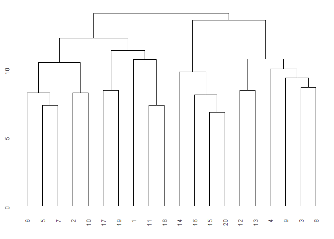
indiv <- "stand"
group <- "Use"

ggdendro::ggdendrogram(cls_add_group(cls, df, indiv, group))
#> Joining with `by = join_by(stand)`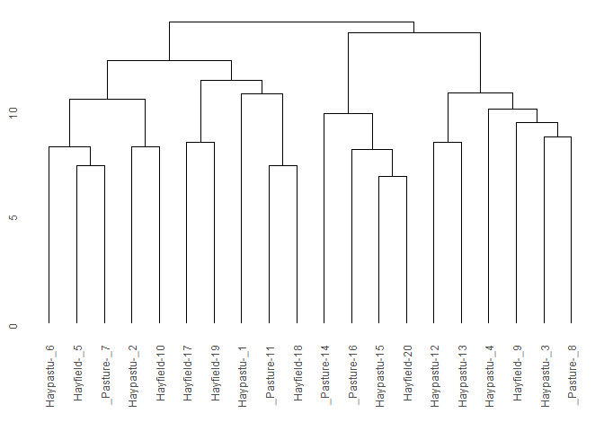
col <- cls_color(cls, df, indiv, group)
#> Joining with `by = join_by(stand)`
#> Joining with `by = join_by(Use)`
cls <-
  cls_add_group(cls, df, indiv, group) %>%
  stats::as.dendrogram()
#> Joining with `by = join_by(stand)`
labels_colors(cls) <- gray(0)

plot(cls)
dendextend::colored_bars(colors = col, cls, group, y_shift = 0,  y_scale = 3)
par(new = TRUE)
plot(cls)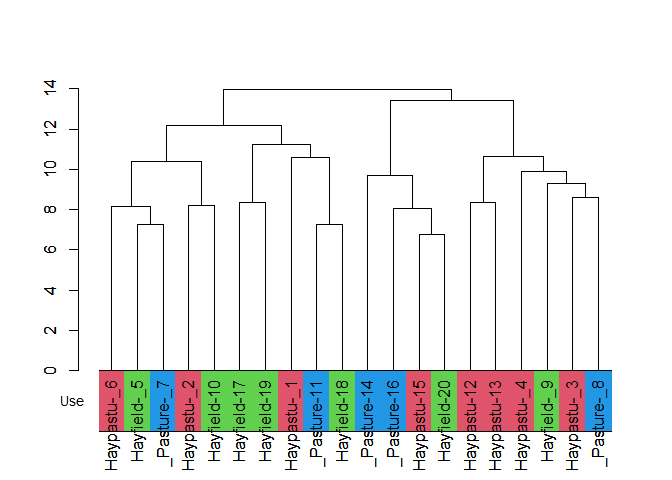
TWINSPAN
twinspan() is a native R implementation of TWINSPAN (Hill 1979) and of the modified TWINSPAN of Roleček et al. (2009). It needs no compiler, but it is not a port of Hill’s original FORTRAN program: see ?twinspan for the known differences.
tw <- twinspan(dune)
tw
#> TWINSPAN
#>   stands:       20
#>   pseudospecies: 75
#>   cut levels:   0 2 5 10 20
#>   divisions:    6
#>   groups:       7
#>
#> division 1 at level 0 (n = 20, eig = 0.511)
#>   indicators: Ranuflam_1(+) Agrostol_1(+) Eleopalu_1(+) Lolipere_1(-)
#> division 2 at level 1 (n = 13, eig = 0.384)
#>   indicators: Hyporadi_1(-)
#> division 3 at level 1 (n = 7, eig = 0.411)
#>   indicators: Sagiproc_1(-)
#> division 4 at level 2 (n = 10, eig = 0.317)
#>   indicators: Planlanc_1(-)
#> division 5 at level 3 (n = 5, eig = 0.284)
#>   indicators: Achimill_1(+)
#> division 6 at level 3 (n = 5, eig = 0.301)
#>   indicators: Juncarti_1(+)

head(tw$classification)
#> # A tibble: 6 × 4
#>   stand group path  depth
#>   <chr> <int> <chr> <int>
#> 1 11        1 00        2
#> 2 17        1 00        2
#> 3 19        1 00        2
#> 4 18        2 0100      4
#> 5 5         3 0101      4
#> 6 6         3 0101      4

# the division tree works with the clustering helpers of ecan
ggdendro::ggdendrogram(stats::as.hclust(tw))
The modified TWINSPAN divides the most heterogeneous group first, so that the number of groups can be chosen directly.
tw_mod <- twinspan(dune, modified = TRUE, n_clusters = 4)
table(tw_mod$classification$group)
#>
#>  1  2  3  4
#>  3 10  3  4
tw_two_way() arranges the stands and the species by their divisions. The digits below the table show the dichotomy of each stand.
tw_two_way(tw)
#>          11115671123498111112
#>          1798   0      234560
#> Cirsarve -----------2--------  0000
#> Elymrepe ----2---22223-------  0000
#> Bellpere ---22--2-222--------  0001
#> Bromhord ----2-22-2-2--------  0001
#> Trifprat ----232-------------  0001
#> Airaprae -22-----------------  00100
#> Empenigr --2-----------------  00100
#> Hyporadi 223-----------------  00100
#> Vicilath 2--1---1------------  00100
#> Achimill -2--222212----------  00101
#> Anthodor -22-2222------------  00101
#> Planlanc 22-23332------------  00101
#> Lolipere 3--22333333322------  0011
#> Poaprat  21-22222223222-2----  0011
#> Rumeacet ----332-----2-2-----  0011
#> Bracruta 2-232322--22222--222  01
#> Poatriv  ----323223333223--2-  01
#> Scorautu 32332222-322222222-2  01
#> Trifrepe 2-222323-321222231--  01
#> Sagiproc 2-2--------32222----  100
#> Salirepe --22---------------3  100
#> Agrostol ----------2322232233  101
#> Alopgeni ---------2322333--2-  101
#> Juncbufo ------2-----2-22----  101
#> Ranuflam -------------2-22222  1100
#> Callcusp ----------------2-22  1101
#> Comapalu ----------------22--  1101
#> Eleopalu -------------2--2332  1101
#> Juncarti ------------22---222  1101
#> Chenalbu ---------------1----  111
#>
#>          00000000000001111111
#>          00011111111110001111
#>             0000011111
#>             0111100001
Ordination
ord_dca <- ordination(dune, o_method = "dca")
ord_pca <-
  df %>%
  df2table() %>%
  ordination(o_method = "pca")

ord_dca_st <-
  ord_extract_score(ord_dca, score = "st_scores")

ord_dca_st %>%
  ggplot(aes(DCA1, DCA2, label = rownames(.))) +
  geom_text()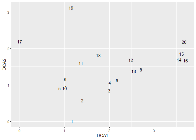
indiv <- "species"
group <- "dammy_1"
ord_pca_sp <-
  ord_add_group(ord_pca, score = "sp_scores", df, indiv, group)
#> Joining with `by = join_by(species)`

ord_pca_sp %>%
  ggplot(aes(PC1, PC2, label = rownames(.))) +
  geom_point(aes(col = .data[[group]]), alpha = 0.4, size = 7) +
  geom_text() +
  theme_bw()
Citation
Toshikazu Matsumura (2022) Ecological analysis tools with R. https://github.com/matutosi/ecan/.